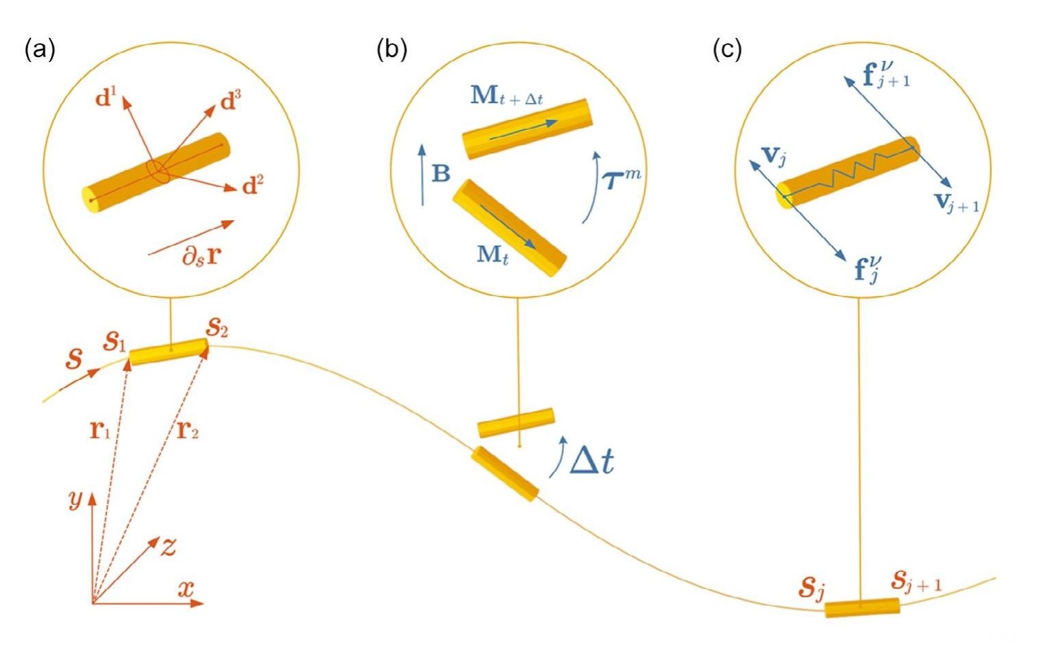
Figure 1. Numerical model of MSRs. a) Cosserat rod model abstracts a slender structure into a centerline curve and cross sections. Positional vector r is used to describe coordinates of nodes under the Eulerian coordinates. A triad of orthogonal vectors {d1,d2,d3} is used to describe the orientation of elemental cross sections. d3 is usually chosen to be perpendicular to the corresponding cross section and is not in the same direction with centerline tangent s ∂ r due to shear. b) Elements in MSRs with magnetization M are driven by magnetic torques τm to be aligned toward the direction of external magnetic field B. M is set to be relatively static with the triad {d1,d2,d3} so the direction of magnetization will move with the motion of elements. c) Elemental damping forces are modeled to be proportional to the difference of speed between nodes in order to eliminate vibration quickly and at the same time make as little influence on rigid body motion.

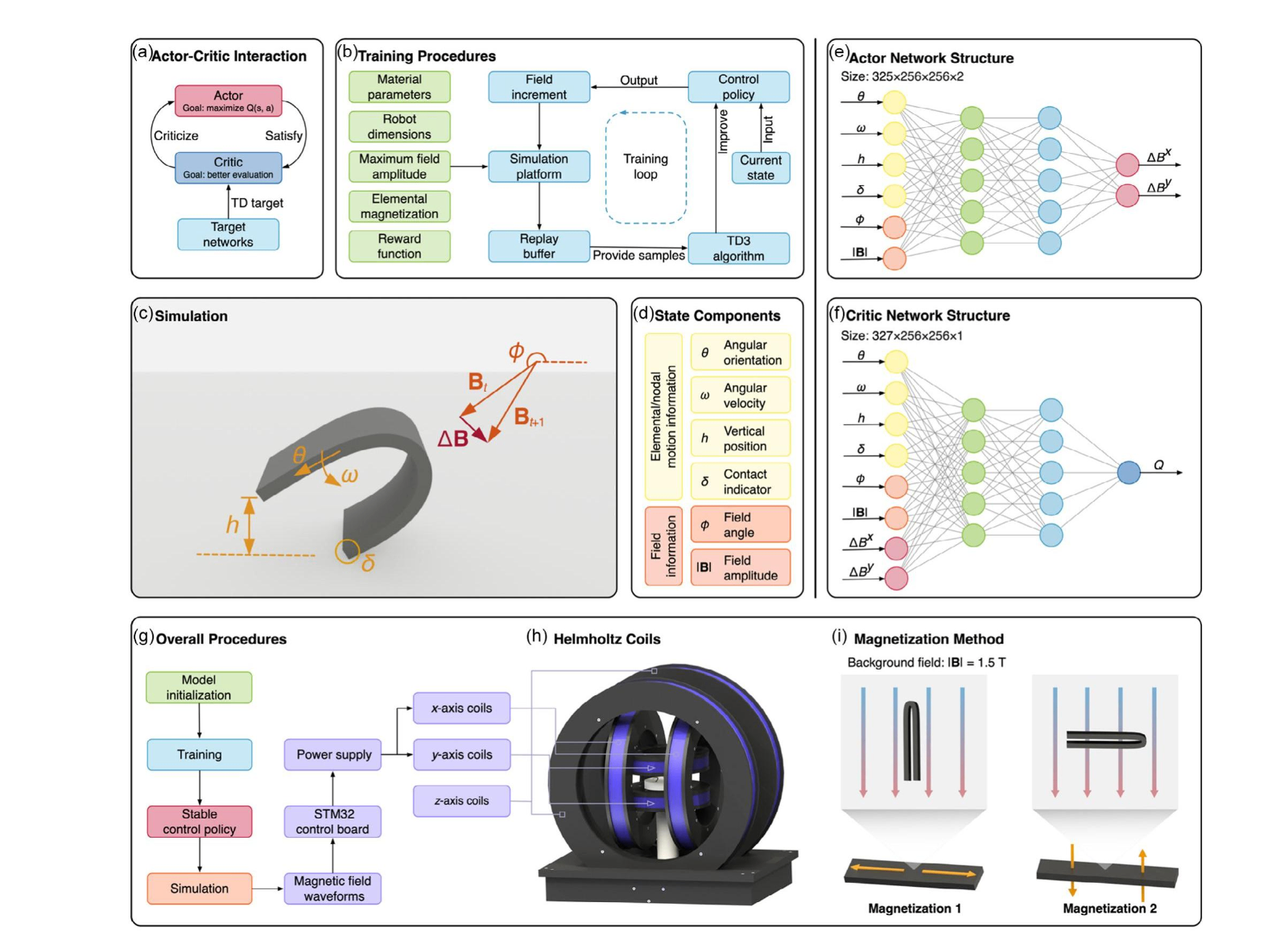
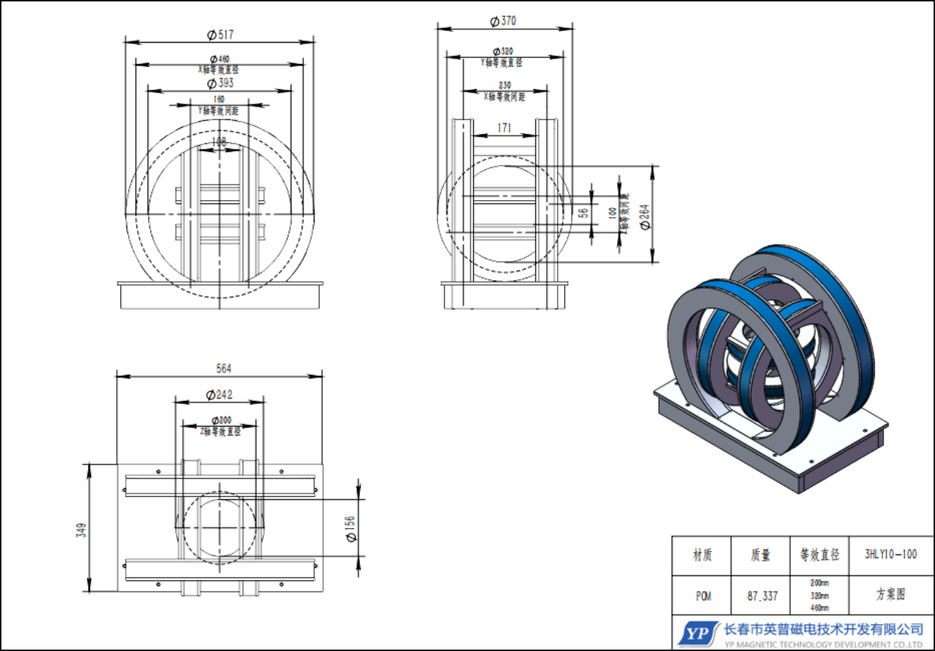
Figure 2. Components and procedures of the RL control system. a) Interaction between different parts of the TD3 algorithm. b) Training procedures for obtaining stable control policies. c) The simulation platform we use. In the picture, we annotate states and actions. In our work, we choose componentsof f ield increment ΔB as actions, and quantities involving necessary information of robot motion or magnetic field are defined as states. d) State variables consisting of angular orientation, angular velocity, vertical position, contact indicator, field angle, and field amplitude. Notice that state variables involving robot motion are defined element-wise or node-wise, so the fineness of segmentation will affect the total size of state variables. e) The structure of the actor network. The actor is used to map states to actions. f) The structure of the critic network. The critic is used to evaluate state-action pairs. g) Overall procedures of our RL control system. After training, we validate the stable control policies in simulations and, at the same time, obtain a set of magnetic f ields. The fields are then used to control the power supply via an STM32 control board. h) Helmholtz coils. For now, we use only two pairs of coils. i) Magnetization method of strip-like soft robots. MSRs presented in our cases are folded and put into a background field in two directions; therefore, robots with two different magnetization patterns are produced.

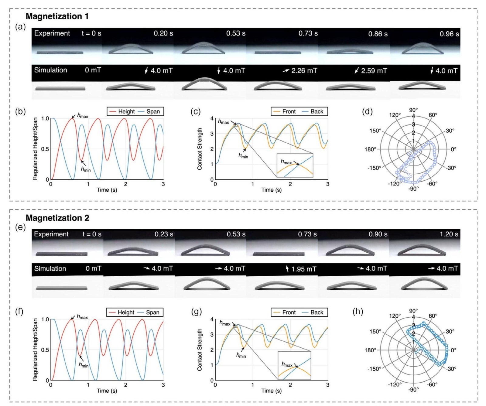
Figure 3. Learning results under relatively small field amplitude. Notice that the plots are from data in simulations. The dimensions of our robots are 20mm 8mm 0.8mm. a) Comparisons between simulation and experiment of the robot with magnetization 1. Directions of magnetic fields are indicated with a white arrow, and amplitudes of fields are annotated in number. The real soft robot reaches its maximum height about 0.3s faster than the simulated one because our dampingmodelleads tosomeoverdampingeffect onrotation, which leads to some mismatch in the comparisons, but overall moving gaits betweenthe two are in goodagreement.SeeMovieS1,SupportingInformation for more. b) Regularized height or span of the robot in 0–3s. Whenthespanreachesitsminimum, theheightreaches itsmaximum,andvice versa.c) Strengthof the front end and the backend contactingthe ground in 0–3s. Whentheheight of therobot reaches a maximum,the contactstrengthof the back end becomes largerthan the front end. d) Scatteredfield plots of applied to the robot in 0–10s. e) Comparisons between simulation and experiment of the robot with magnetization 2. See Movie S2, Supporting Information for more. f–h) The plots of the robot with magnetization 2 corresponding to (b–d). The learned moving gait is very similar to the one of magnetization 1. Two scattered plots of fields share similar contour shapes but have different orientations, which indicates similar torques among the two robots.

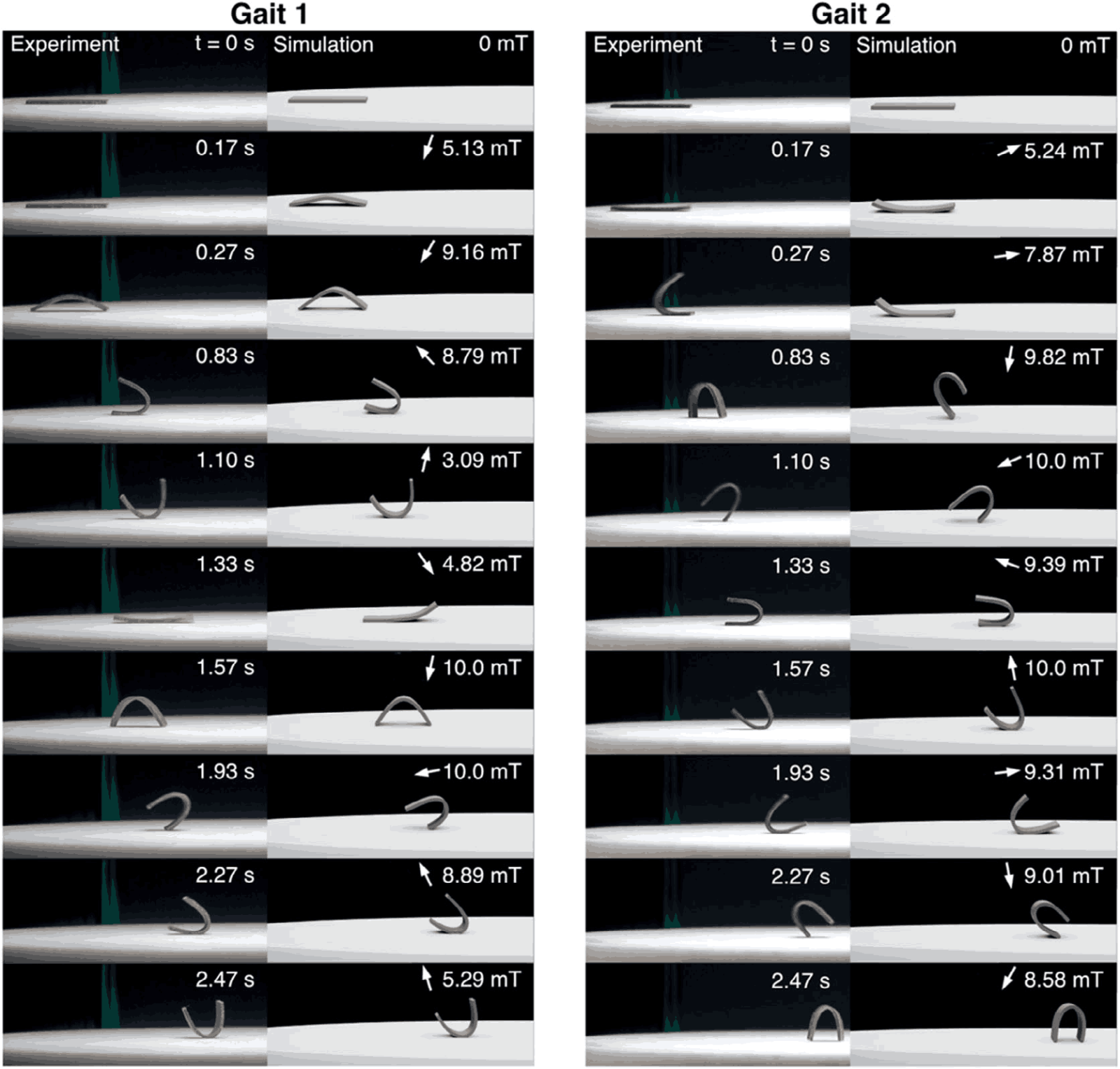
Figure 4. Comparisons between simulations and experiments of the robot with magnetization 1 under relatively large fields. Two different gaits are learned due to run-to-run variances of TD3. The experiments show good agreements with simulations with the exception of highly dynamic conditions at the beginning of gait 2 due to overdamping on rotations. See Movie S3 and S4, Supporting Information for more.

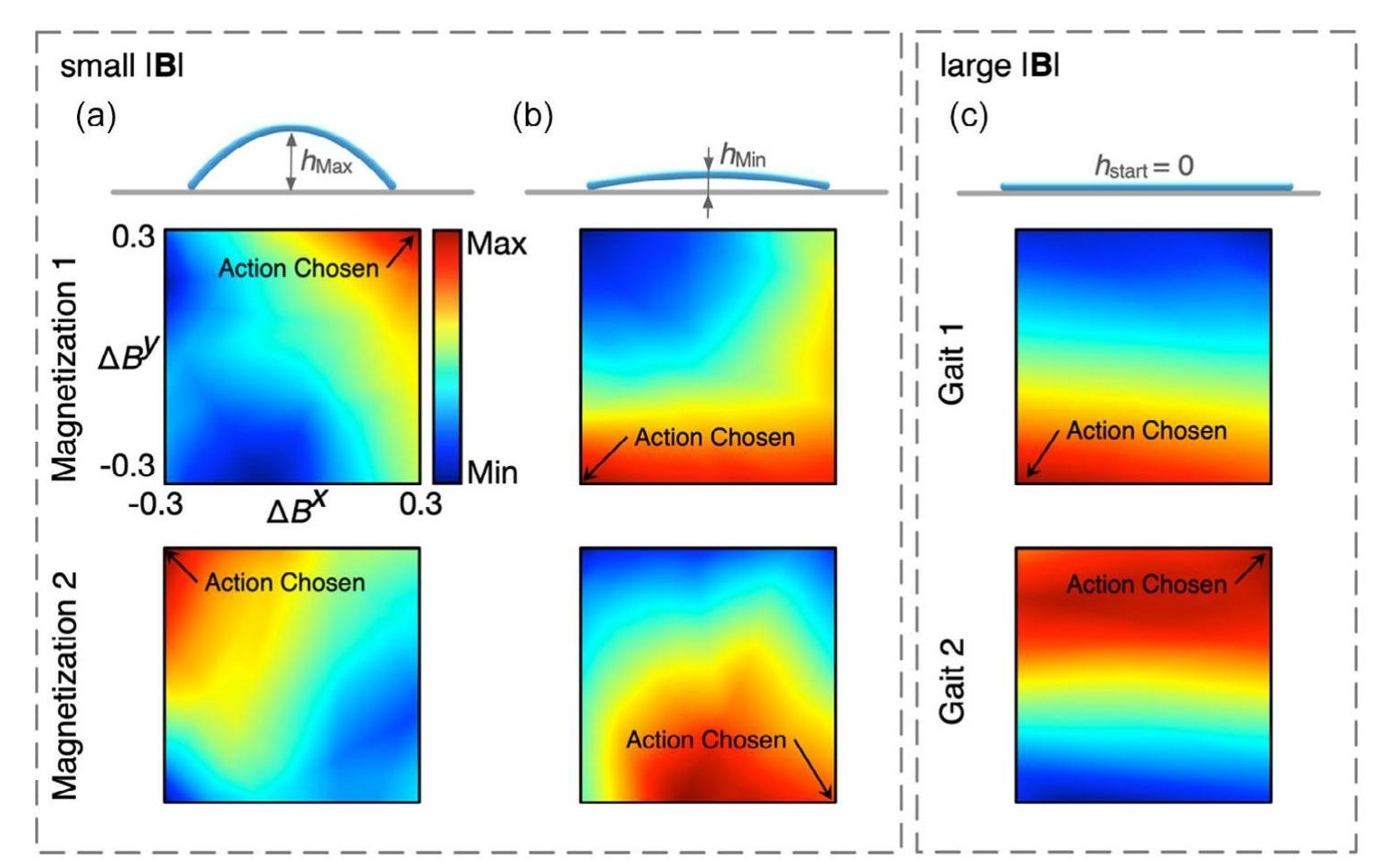
Figure 5. Q-value distributions for different actions estimated by different agents. We get these heat maps by inputting uniformly distributed actions to critics under certain states. The axes are in the unit of mT. In the plots, the points annotated by “Action Chosen” are the actual field increment chosen by actors. a) Q-value distributions when robots reach their highest point. Two agents trained under different magnetization patterns both choose different actions that correspond to points with a maximum Q-value. b) Q-value distributions when robots reach their lowest point. The action selected by the agent of magnetization 2 does not have the highest Q-value. c) Q-value distributions of agents corresponding to two gaits are shown in Figure 4. We choose the specific state to be at the starting position because it is shared by both gaits.